This week, I was lucky enough to work at the EISCAT Svalbard
Radar, where I was able to run experiments and also be involved with designing
and running a new experiment. EISCAT runs incoherent scatter radars north of
the Arctic circle in three countries (Finland, Norway and Sweden). The radars
take measurements of the terrestrial ionosphere and atmosphere. One of these
radars is located on Svalbard, around 15 km from the main town, Longyearbyen.
The EISCAT Svalbard Radar (ESR) operates at 500MHz, and consists of two dishes;
a 42m field aligned antenna, and a 32m moveable antenna.
On our first evening at ESR, we were given the task of
making our own antenna using tin can, thus, making ‘cantennas’. The first step
was to choose the perfect can for our cantenna. The tin cans are short circular
waveguides that can be used as antennas that will work at certain frequency
ranges. Our desired frequency range was 2.4-2.48GHz, and so using this and
measuring the diameters of the tin cans, we could then calculate the cutoff
frequencies for each can and determine which one would work for our frequency
range. The ‘fruit cocktail’ tin can was chosen to be made into an antenna. Once
we had the right sized can, we then had to determine the location of the feed
into the waveguide, and the length of the monopole. The monopole is a single
wire and is feed directly into the waveguide (the tin can). The length of the
monopole needs to be a quarter of the wavelength in free air. We marked this
length on the wire, and cut the wire to a cm more than the desired length to
allow for fine tuning the wire later. The monopole then needs to be fed into
the can at a specific distance from the back wall of the can. This distance is
a quarter of the wavelength inside the waveguide. After many calculations we
made markings on the can of the centre of the back wall, and of where the
monopole would be fed in. Holes were drilled into these two locations such that
the monopole was fed into the can, and the can could be screwed to a plank
ready for testing at a later date.

On the second evening, my group (myself, Brad and Magnus)
ran our own experiment on the ESR. The klystrons are turned on in the
transmitter room where the power that’s transmitted is generated (typically
MWatts of power). The power is then released in bursts, ‘pulses’ into the sky,
alternatively between the 32m and the 42m. Our experiment was designed in order
to look for polar cap patches; localized density enhancements in the ionosphere
that enter that polar cap at the dayside cusp and convect into the nightside,
exiting the polar cap near midnight. Signatures of polar cap patches can mainly
be seen in the electron density and ion drift velocity measured by ESR. In
addition to ESR, we would be using SuperDARN and DSCOVR data to observe the
convection speeds and the IMF-Bz respectively. The 42m dish is fixed and points
field aligned (184.5˚, 81.6˚), whilst we set the 32m dish to
perform an azimuthal scan. The azimuthal scan scanned to the North East of
Svalbard from 0-120˚ azimuth
at an elevation of 30˚.
To operate the ESR, a tool called EROS (command line based)
is used to start, run and stop experiments, as well as starting and stopping
recording of data and changing the position of the antenna. The real-time
performance of the radar is monitored using the program RTG which shows various
parameters such as the raw data dump, time and elevation/azimuth. A tool called
TRIL is then used to monitor interlocks and transmitter status. TRIL is used to
put the klystrons in four different modes; in black heat mode the klystrons are
powered up so that they are ready for transmit. Just before transmitting,
Standby mode is used such that the klystrons are ready to transmit within a
couple of seconds. In Transmit mode the power is transferred through the
waveguides and to the antenna. The Off mode is then used when the radar is
being switched off for a long time. The
experiment can then be started in the EROS command window by specifying the
location of the experiment elan files, the time start of the experiment, the
scan file for the dishes and the ID of the country running the experiment. Once
the experiment is running, the real time data can be observed by loading the
RTG plots, and analysed using Guisdap. The RTG plots show the pulses of the 32m
and 42m. Plots of the raw electron density, electron temperature, ion
temperature, ion velocity and radar parameters are then loaded in Guisdap.
During our experiment, there was very little ionosphere and so no polar caps
were observed. However, we learned valuable skills in operating and running
ESR, reading and analysing real time raw data. This data will be further
analysed, alongside other data obtained from ESR in Matlab at a later date.


On the third evening at ESR, we continued with our cantenna
designs, and designed a new experiment for the ESR. With the cantenna, we fine
tuned the monopole; this involved cutting small amounts off the monopole and
until it was transmitting at an optimum. We then worked together to design an
experiment such that the ESR 32m dish scanned the same area of the ionosphere
as SuperDARN. SuperDARN is a high frequency coherent scatter radar, and there
is more than 30 of these radars in both the northern and southern hemisphere.
One of these is located on Svalbard, and is a new radar beginning operations in
October 2016. With numerous calculations and discussions, and experiment was
ready to be tested the following day.
On the fourth evening, we were set to test our new
experiment. The 32m dish was set to perform an azimuthal scan from 231.24-179.4˚ at a 150˚ elevation. SuperDARN always has 16 beams in a scan, each with
a 3.24˚ separation, so in
order to match the scan as closely as possible to ESR, an 8 second dwell was
required for each beam. With both ESR and SuperDARN set up, the new experiment
begun. It was shortly found that the 32m period had been set incorrectly, this
was quickly altered and attempts were made to re-sync ESR with SuperDARN. This
was unsuccessful, and so the experiment had to be re started. On restarting
however, the experiment was doing exactly what we had desired it to and
numerous structures were observed for further analysis.


Our final evening at ESR, we put our cantennas to the test.
We set up two of the best cantennas to transmit our desired frequency, and then
a signal is received. We had many people running to and from the cantennas, drove
a car to and from then cantenna, and even attempted to interpret a plasma
bubble. The spectrum of moving bodies can then be seen on via a programme on
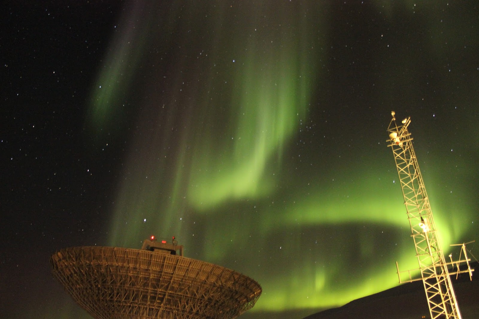
the computer. Then, after a long week of no aurora, we finally got some
beautiful aurora which looked stunning as it danced above the two antennas. A
wonderful end to a wonderful week!!
 |
| Testing the Cantennas |

 |
| Aurora over 42m dish |
 |
| Aurora over 32m dish |
Between my last blog and this blog, I have done lots of
different things in and around Longyearbyen, so stay tuned for the next blog
and video coming very soon, ‘Life on Svalbard’!! Hope you enjoy the video that accompanies
this blog too.
Ser deg seinare!
No comments:
Post a Comment